This time write a Logistic Regression module. And, unlike in the Linear Regression post, we will let numpy generate data for us. Also, we will look use some basic plotting.
Let’s get started.
1
2
3
4
5
6
7
8
9
10
11
12
13
14
15
16
17
18
19
20
21
22
23
24
25
26
27
28
29
30
31
32
33
34
35
36
37
38
39
40
41
42
43
44
45
46
47
48
49
50
51
52
53
54
55
56
57
58
59
60
61
62
63
import numpy as np
import torch
from torch import nn
from torch.autograd import Variable
from torch import optim
import torch.nn.functional as F
# For plotting
import matplotlib.pyplot as plt
import seaborn as sn
from pylab import rcParams
NUM_EPOCHS = 10
sn.set_style('darkgrid') # Set the theme of the plot
rcParams['figure.figsize'] = 18, 10 # Set the size of the plot image
# Creating a Logisitic Regression Module
# which just involves multiplying a weight
# with the feature value and adding a bias term
class LogisticRegression(nn.Module):
def __init__(self):
super(LogisticRegression, self).__init__()
# Since there is only a single feature value,
# and the output is a single value, we use
# the Linear module with dimensions 1 X 1.
# It adds a bias term by default
self.linear = nn.Linear(1, 1)
def forward(self, x):
return F.sigmoid(self.linear(x))
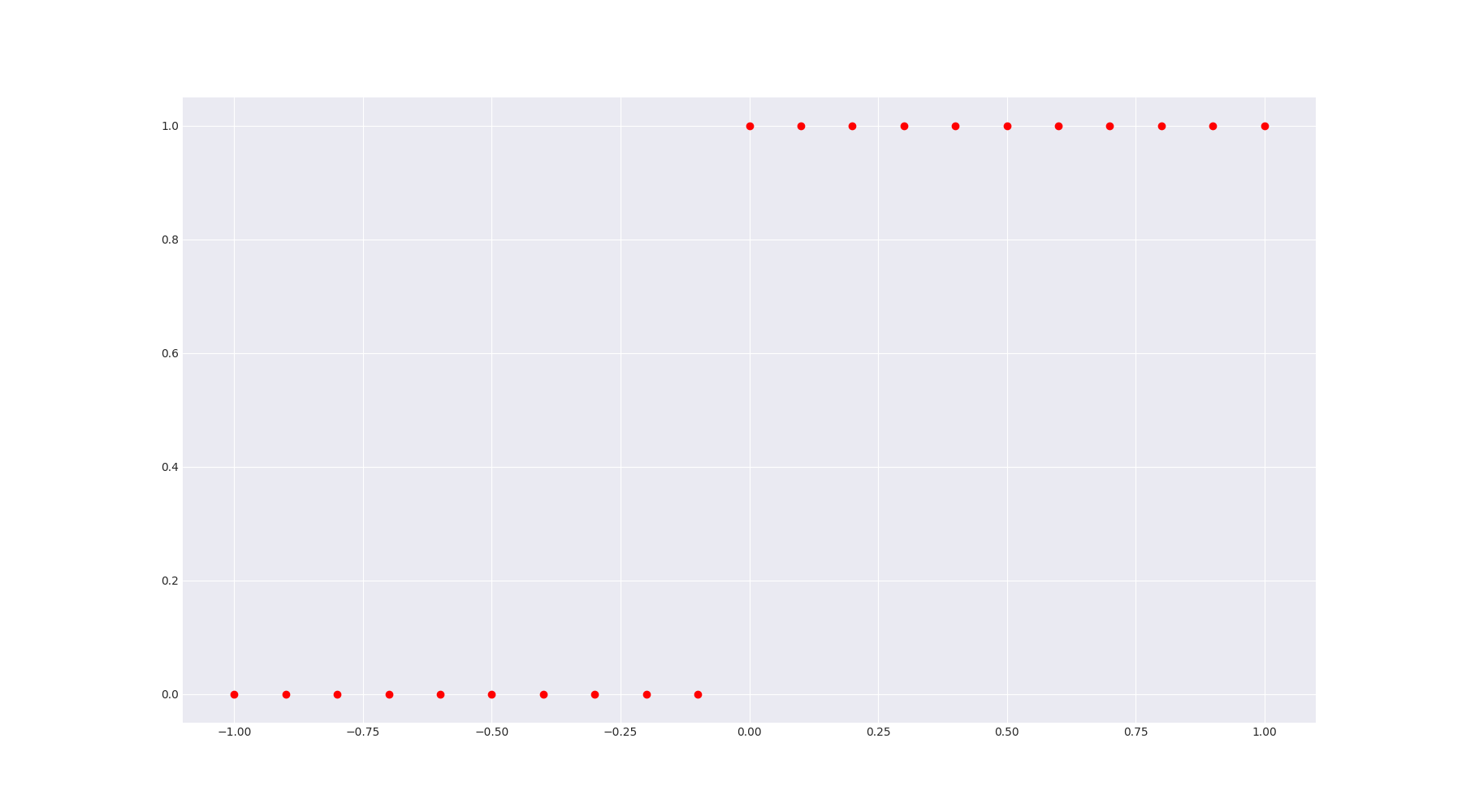
# Preparing data for classification
xs = np.linspace(-1, 1, 21)
ys = np.array([0.0 if x < 0 else 1 for x in xs])
# Plot the points to see if everything is right
plt.plot(xs, ys, 'ro')
plt.show()
# We use torch's `from_numpy` function to convert
# our numpy arrays to Tensors. They are later wrapped
# in torch Variables
x = Variable(torch.from_numpy(xs), requires_grad=False)
y_true = Variable(torch.from_numpy(ys), requires_grad=False)
logreg = LogisticRegression()
criterion = nn.BCELoss() # Using the Binary Cross Entropy loss
# since it's a classfication task
optimizer = optim.SGD(logreg.parameters(), lr=0.1)
for i in range(NUM_EPOCHS):
y_pred = logreg(x)
loss = criterion(y_pred, y_true)
print('Loss:', loss.data, 'Parameters:',
list(map(lambda x: x.data, logreg.parameters())))
optimizer.zero_grad()
loss.backward()
optimizer.step()
Upon running the code above, we first get this plot:
And then the trace below:
1
2
3
4
5
6
7
8
9
10
11
12
13
14
Traceback (most recent call last):
  File "/media/saqib/ni/Projects/PyTorch_Practice/LogisticRegression.py", line 56, in <module>
    y_pred = logreg(x)
  File "/usr/local/lib/python3.6/site-packages/torch/nn/modules/module.py", line 491, in __call__
    result = self.forward(*input, **kwargs)
  File "/media/saqib/ni/Projects/PyTorch_Practice/LogisticRegression.py", line 32, in forward
    return F.sigmoid(self.linear(x))
  File "/usr/local/lib/python3.6/site-packages/torch/nn/modules/module.py", line 491, in __call__
    result = self.forward(*input, **kwargs)
  File "/usr/local/lib/python3.6/site-packages/torch/nn/modules/linear.py", line 55, in forward
    return F.linear(input, self.weight, self.bias)
  File "/usr/local/lib/python3.6/site-packages/torch/nn/functional.py", line 994, in linear
    output = input.matmul(weight.t())
RuntimeError: Expected object of type torch.DoubleTensor but found type torch.FloatTensor for argument #2 'mat2'
What happend? Well, PyTorch actually uses FloatTensor objects for model weights and biases. There are two ways to get around this. We can either convert our inputs and outputs to FloatTensor objects or convert our model to DoubleTensor. Either of it should work, but I did a little bit of digging around on PyTorch Forums and Stackoverflow and found that computations on doubles are less efficient. So, we will stick with converting our data to FloatTensor objects.
So we add the lines below to our code, after we have created the Variable objects, on lines 46 and 47 and try running it again:
1
2
x = x.float()
y_true = y_true.float()
When we run this, however, we run into another exception:
1
2
3
4
5
6
7
8
9
10
11
12
13
14
Traceback (most recent call last):
  File "/media/saqib/ni/Projects/PyTorch_Practice/LogisticRegression.py", line 58, in <module>
    y_pred = logreg(x)
  File "/usr/local/lib/python3.6/site-packages/torch/nn/modules/module.py", line 491, in __call__
    result = self.forward(*input, **kwargs)
  File "/media/saqib/ni/Projects/PyTorch_Practice/LogisticRegression.py", line 32, in forward
    return F.sigmoid(self.linear(x))
  File "/usr/local/lib/python3.6/site-packages/torch/nn/modules/module.py", line 491, in __call__
    result = self.forward(*input, **kwargs)
  File "/usr/local/lib/python3.6/site-packages/torch/nn/modules/linear.py", line 55, in forward
    return F.linear(input, self.weight, self.bias)
  File "/usr/local/lib/python3.6/site-packages/torch/nn/functional.py", line 994, in linear
    output = input.matmul(weight.t())
RuntimeError: size mismatch, m1: [1 x 21], m2: [1 x 1] at /pytorch/aten/src/TH/generic/THTensorMath.c:2033
What happend this time? The error message says that the size of the tensors does not match. Okay, let’s check. Well, the size of x, seems correct \(1 \times 23\), but how come y has dimensions \(1 \times 1\)? You see, the problem is that PyTorch and even other libraries like scikit-learn expect a feature matrix. Howerver, ours is a vector with \(23\) dimensions. In case where the number of features is more than 1, we would provide a matrix indeed. But, for our case here, creating a \(1 \times 23\) is ambiguous. Does it represent a single data point with \(23\) features or \(23\) data points with \(1\) feature each? Therefore, we will convert our vectors into matrices by calling .reshape(-1, 1) on each of them.
So, our code now becomes:
1
2
3
4
5
6
7
8
9
10
11
12
13
14
15
16
17
18
19
20
21
22
23
24
25
26
27
28
29
30
31
32
33
34
35
36
37
38
39
40
41
42
43
44
45
46
47
48
49
50
51
52
53
54
55
56
57
58
59
60
61
62
63
64
65
66
67
68
import numpy as np
import torch
from torch import nn
from torch.autograd import Variable
from torch import optim
import torch.nn.functional as F

# For plotting
import matplotlib.pyplot as plt
import seaborn as sn
from pylab import rcParams

NUM_EPOCHS = 10

sn.set_style('darkgrid')    # Set the theme of the plot
rcParams['figure.figsize'] = 18, 10  # Set the size of the plot image

# Creating a Logisitic Regression Module
# which just involves multiplying a weight
# with the feature value and adding a bias term
class LogisticRegression(nn.Module):

    def __init__(self):
        super(LogisticRegression, self).__init__()
        # Since there is only a single feature value,
        # and the output is a single value, we use
        # the Linear module with dimensions 1 X 1.
        # It adds a bias term by default
        self.linear = nn.Linear(1, 1)

    def forward(self, x):
        return F.sigmoid(self.linear(x))


# Preparing data for classification
xs = np.linspace(-1, 1, 21)
ys = np.array([0.0 if x < 0 else 1 for x in xs])

# Plot the points to see if everything is right
plt.plot(xs, ys, 'ro')
plt.show()

# We use torch's `from_numpy` function to convert
# our numpy arrays to Tensors. They are later wrapped
# in torch Variables
x = Variable(torch.from_numpy(xs), requires_grad=False)
y_true = Variable(torch.from_numpy(ys), requires_grad=False)

x = x.float()
y_true = y_true.float()

# Convert to feature matrices
x = x.reshape(-1, 1)
y_true = y_true.reshape(-1, 1)

logreg = LogisticRegression()
criterion = nn.BCELoss()   # Using the Binary Cross Entropy loss
                           # since it's a classfication task
optimizer = optim.SGD(logreg.parameters(), lr=0.1)

for i in range(NUM_EPOCHS):
    y_pred = logreg(x)
    loss = criterion(y_pred, y_true)
    print('Loss:', loss.data, 'Parameters:',
          list(map(lambda x: x.data, logreg.parameters())))
    optimizer.zero_grad()
    loss.backward()
    optimizer.step()
On running this code now, we get the following output:
1
2
3
4
5
6
7
8
9
10
Loss: tensor(1.0144) Parameters: [tensor([[-0.9143]]), tensor([ 0.7357])]
Loss: tensor(1.0013) Parameters: [tensor([[-0.8810]]), tensor([ 0.7216])]
Loss: tensor(0.9885) Parameters: [tensor([[-0.8479]]), tensor([ 0.7077])]
Loss: tensor(0.9758) Parameters: [tensor([[-0.8150]]), tensor([ 0.6940])]
Loss: tensor(0.9634) Parameters: [tensor([[-0.7823]]), tensor([ 0.6805])]
Loss: tensor(0.9512) Parameters: [tensor([[-0.7499]]), tensor([ 0.6673])]
Loss: tensor(0.9391) Parameters: [tensor([[-0.7176]]), tensor([ 0.6543])]
Loss: tensor(0.9273) Parameters: [tensor([[-0.6856]]), tensor([ 0.6415])]
Loss: tensor(0.9157) Parameters: [tensor([[-0.6539]]), tensor([ 0.6290])]
Loss: tensor(0.9043) Parameters: [tensor([[-0.6223]]), tensor([ 0.6166])]
We can the the loss going down. You can change the number of epochs by changing the vale of the variable NUM_EPOCHS, to decrease the loss further.
I ran the model for 2000 epoch and used the following code snippet to draw a decision boundary for my model:
1
2
3
4
5
6
7
8
9
params = list(map(lambda x: x.data, logreg.parameters()))
m = params[0].numpy()[0][0]
c = params[1].numpy()[0]
print(m, c)
y = m * x.numpy() + c
plt.plot(xs[np.where(xs >= 0)], ys[ys == 1.0], 'bo')
plt.plot(xs[np.where(xs < 0)], ys[ys == 0.0], 'ro')
plt.plot(x.numpy(), y, 'g')
plt.show()
This is what I got:
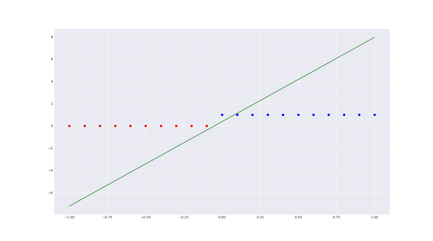
The decision boundary in green misclassifies one point. We can train it more to improve the performance futher.
Comments